Uncertainty Quantification
Meet the researchers in uncertainty quantification, using statistical modelling not only to make predictions about complex real-world systems, but to tell us how confident we can be in the answers.
Our world is full of complicated systems, where lots of factors interact. Think of a disease like covid-19, where the number of infected people, local geography, government rules and many more factors will influence a quantity like the number of people going to hospital.
To predict what will happen next, and to understand the system, we use computer simulators. We summarise the state of things by a collection of numbers we call ‘input parameters’. In the covid-19 example, these might include things like the incubation period, how long people remain infectious for, what proportion of people follow the government guidelines and so on. There are often hundreds of parameters, aiming to capture (in a simplified form) the state of the system.
The simulator uses these input parameters in some mathematical functions (written by experts, in this case epidemiologists) to calculate an ‘output variable’, for example daily hospitalisations. We call the collection of functions the ‘model’, because it is a simplified representation of reality.

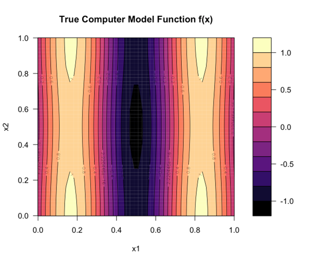
Figure 1: This simulator has two input variables, x1 and x2, each between 0 and 1. For each possible pair it calculates an output which is shown by a colour from purple to yellow. For example if x1 is 0.2 and x2 is 0.6, the output is just below 1.
This framework is very general. The Uncertainty Quantification group at Durham have worked with simulators of many systems, including:
- Galaxy formation
- Rainfall runoff and flooding
- Gas/Oil pipeline damage
- Climate
- Ocean ecosystems
- Energy networks
- Epidemics
- Nuclear physics
While each area has its own scientific questions, there are always certain challenges around using simulators to understand and predict the real world.
We don’t know the ‘true’ values of the input parameters. First, we can rarely measure them directly. In our covid-19 example, how would we measure the exact duration over which someone is infectious? Even if we could, the duration would vary for different people, so there is no ‘true’ value. This means we can’t just run the simulator once: we might suggest a few sensible values for each input, and run the simulator at combinations of those values to get an idea of the values the output might take.
The model in the simulator can be so complex that the simulator might take several hours, or even days, to run and produce the output. Suppose our simulator has 10 inputs (a very small number!) and we choose three ‘sensible’ values for each of these. This gives us 3 x 3 x … x 3 = 3^10, or around 59,000 possible combinations. If the simulator takes 1 hour to run, then it would take us almost 7 years to run it for all these input combinations!
This is where emulation and uncertainty quantification come in. An emulator is a statistical model of the simulator, that uses data (input and output values) from a relatively small number of simulator runs to learn about the simulator’s output for any combination of input values. Rather than just give one output value, the emulator gives both a ‘best estimate’ and a measure of how uncertain it is about that value.
The basic structure of an emulator is:
function of inputs + correlated noise
- The ‘function of inputs’ part captures the broad behaviour of the simulator as each of the input values changes. Some inputs might have a big effect on the output, while others don’t make much difference.
- The ‘correlated noise’ represents how ‘smooth’ or ‘rough’ the simulator’s output is: how quickly the output changes as the input values change. This determines the emulator’s confidence about the simulator’s output at new input values, and ensures that the emulator can fully reflect data from the simulator.
In general, for new input values that are close to sets of inputs for which we know the simulator’s output, the emulator will be more confident. For input points that are not close to any known point, the emulator will have a lot of uncertainty.

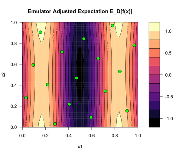
Figure 2: An emulator's prediction for the simulator in Figure 1. We know the simulator's output for the points in green. The emulator has filled in what it thinks is the most likely output value everywhere else.

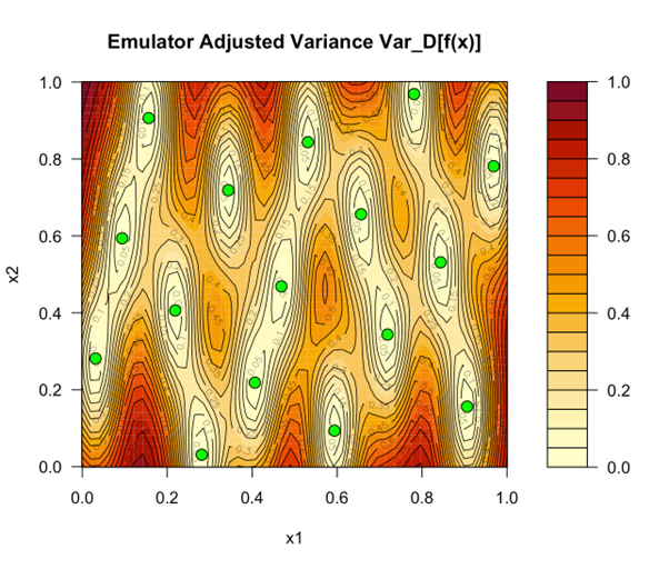
Figure 3: The emulator uncertainty. For the green points the simulator's output is known, so the emulator's uncertainty is zero. In between, the uncertainty goes up.
The emulator runs quickly, so we can use it to answer questions like “which input values are most likely to be ‘true?” or “what would the simulator’s output be for these new input values?”.

The emulator can incorporate other sources of uncertainty, such as the ‘model discrepancy’. This is the difference between the simulator’s output and the corresponding real world value. Even the simulator itself is an approximation of the real-world system; even at the ‘best’ values of the input parameters, the simulator’s output won’t equal the true system value. By accounting for the model discrepancy in our emulator, we can make robust predictions about the real world, even though the simulator is “not true”. By ‘robust’, we mean that the emulator’s prediction and uncertainty reflect as honestly as possible all the understanding we have from the simulator data and from what we know of the difference between the simulator and the real world.
The group in Durham has played a leading part in the field of uncertainty quantification since the outset, around 30 years ago. Some questions we’ve recently been working on are:
- How can we learn from multiple simulators of the same system?
- How can scientific insight enable the emulator to learn about the simulator more effectively?
- Can a more sophisticated treatment of model discrepancy increase the robustness of our predictions?
- How do we use emulators to help organisations make decisions?
The progress made by the UQ group at Durham has impacted multiple scientific areas.
Find out more:
- Discovering a new isotope of oxygen (full Nature article, news and views)
- Examining the nucleus of lead atoms (full Nature physics article, news and views)
- An investment case for new tuberculosis vaccines (WHO report)

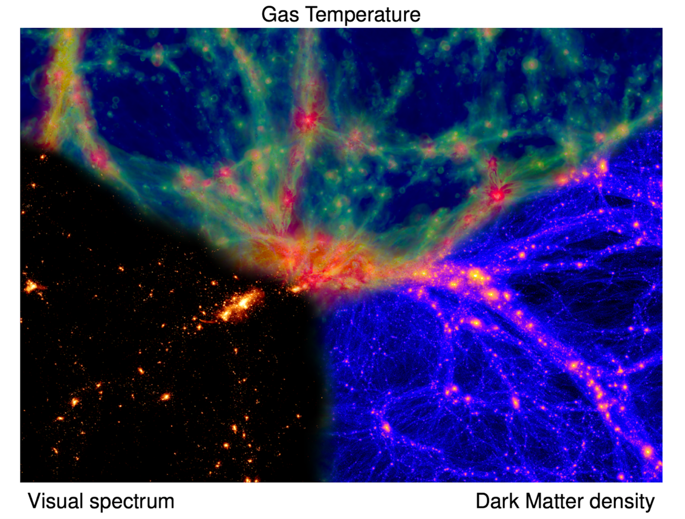
Figure 4: An example of a Galaxy formation simulation known as EAGLE. It simulates the formation and growth of millions of galaxies from soon after the Big Bang until the current day. Emulating such a model is extremely useful but also very challenging.
Meet the experts
Meet our experts in Uncertainty Quantification, driving real-world impact by simulating outcomes across diverse fields, from galaxy formation and climate change to ecosystems, nuclear physics, and epidemics.
Scroll to view all faces
Discover new faces
Explore our other 100 Faces of Science themes and discover the incredible stories of people making a real-world impact across a wide range of fields. From sustainability and quantum research to AI and energy, each theme highlights the diverse talent driving innovation at Durham University.


/prod01/prodbucket01/media/durham-university/90535-(1).jpg)
.png)
/prod01/prodbucket01/media/durham-university/UnQuant_MGoldstein.jpg)
/prod01/prodbucket01/media/durham-university/UnQuant_IVernon.jpeg)
/prod01/prodbucket01/media/durham-university/UnQuant_ROughton.jpg)
/prod01/prodbucket01/media/durham-university/UnQuant_SJackson.jpg)
/prod01/prodbucket01/media/durham-university/UnQuant_ZLi.jpg)
/prod01/prodbucket01/media/durham-university/UnQuant_MHasan.jpg)
/prod01/prodbucket01/media/durham-university/UnQuant_SCooper.jpg)
/prod01/prodbucket01/media/durham-university/UnQuant_LParry.jpg)
/prod01/prodbucket01/media/durham-university/UnQuant_AIskauskas.jpeg)